Blog Toán Học Ứng Dụng

Tháng Mười Hai 15, 2009

Khai triển Taylor – Maclaurin

Filed under: Giải tích — Thẻ:Maclaurin, Taylor — tranthevu @ 11:09 sáng

1. Công thức khai triển:

Giả thiết hàm số y = f(x) có tất cả các đạo hàm đến cấp n + 1 (kể cả đạo hàm cấp n + 1) trong một khoảng nào đó chứa điểm x = a.

Hãy xác định một đa thức $y = P_n(x)$ bậc n mà giá trị của nó tại x = a bằng giá trị f(a) và giá trị của các đạo hàm đến hạng n của nó bằng giá trị của các đạo hàm tương ứng của hàm số f(x) tại điểm đó. Nghĩa là:

$P_n(a) = f(a) ; P_{n}^{'}(a) = f'(a);...; P_{n}^{(n)}(a) = {{f}^{(n)}}(a)$ (1)

Ta hy vọng sẽ tìm được một đa thức như thế trong một ý nghĩa nào đó “gần” với hàm số f(x).

Ta sẽ xác định đa thức đó dưới dạng một đa thức theo lũy thừa (x – a) với các hệ số cần xác định:

${{P}_{n}}(x)={{C}_{0}}+{{C}_{1}}.(x-a)+{{C}_{2}}.{{(x-a)}^{2}}+...+{{C}_{n}}.{{(x-a)}^{n}} \qquad$ (2)

Các hệ số $C_0, C_1, C_2, ..., C_n$ được xác định sao cho điều kiện (1) được thỏa mãn.

Trước hết, ta tìm các đạo hàm của $P_n(x)$ :

$\left\{ \begin{array}{l} P_{n}^{'}(x) = C_1 + 2C_2(x-a) + 3C_3.{(x-a)}^2 + ... + nC_n{(x-a)}^{n-1} \\ P_{n}^{''}(x) = 2C_2+3.2C_3.(x-a) + ... + n(n-1)C_n{(x-a)}^{n-2} \\ .................................................................................. \\ P_{n}^{(n)}(x) = n(n-1)...2.1.C_n \\ \end{array} \right.$ (3)

Thay x = a vào các biểu thức (2) và (3) ta có:

$\left\{\begin{array}{l} P_n(a) = C_0 \\ P_n^{'}(a) = C_1 \\ P_n^{''}(a) = 2.1.C_2 \\ \text{....................................} \\ P_n^{(n)}(a) = n.(n-1)...2.1C_n \\ \end{array} \right.$

So sánh với điều kiện (1) ta có:

$\left\{ \begin{array}{l} f(a)={{C}_{0}} \\ f'(a)={{C}_{1}} \\ f''(a)=2.1.{{C}_{2}} \\ ....................... \\ {{f}^{(n)}}(a)=n.(n-1)...2.1.{{C}_{n}} \\ \end{array} \right.$ $\Rightarrow \left\{ \begin{array}{l} {{C}_{0}}=f(a) \\ {{C}_{1}}=f'(a) \\ {{C}_{2}}={ \dfrac{1}{2!}}.f''(a) \\ ....................... \\ {{C}_{n}}={ \dfrac{1}{n!}}.{{f}^{(n)}}(a) \\ \end{array} \right.$ (4)

Thay các giá trị của $C_0, C_1, C_2, ..., C_n$ vào công thức (2) ta có đa thức cần tìm:

$\begin{array}{r}P_n(x) = f(a) + { \dfrac{f'(a)}{1!}}(x-a) + { \dfrac{f''(a)}{2!}}(x-a)^2 + { \dfrac{f'''(a)}{3!}}(x-a)^3 + \\ ... + { \dfrac{f^{(n)}(a)}{n!}}(x-a)^n \\ \end{array}$

Ký hiệu bằng $R_n(x)$ , hiệu giữa giá trị của hàm số đã cho f(x) và đa thức mới lập $P_n(x)$ (hình vẽ): ${{R}_{n}}(x) = f(x) - {{P}_{n}}(x)$

Hay:

$\begin{array}{r} f(x) = f(a) + { \dfrac{f'(a)}{1!}}(x-a) + { \dfrac{f''(a)}{2!}}{{(x-a)}^{2}} + { \dfrac{f'''(a)}{3!}}{{(x-a)}^{3}} + ... \\ + { \dfrac{{{f}^{(n)}}(a)}{n!}}{{(x-a)}^{n}} + {{R}_{n}}(x) \\ \end{array}$ (6)

taylor $R_n(x)$ gọi là số hạng dư – đối với những giá trị x làm cho số hạng dư $R_n(x)$ bé, thì khi đó đa thức $P_n(x)$ cho biểu diễn gần đúng của hàm số f(x).

Do đó, công thức (6) cho khả năng thay hàm số y = f(x) bằng đa thức $P_n(x)$ với độ chính xác tương ứng bằng giá trị của số hạng dư $R_n(x)$

Ta sẽ xác định những giá trị x để số hạng dư $R_n(x)$ khá bé .

Viết số hạng dư dưới dạng: ${{R}_{n}}(x) = { \dfrac{{{(x-a)}^{n+1}}}{(n+1)!}}Q(x)$ (7)

Trong đó Q(x) là hàm số cần phải xác định.

Với x và a cố định, hàm số Q(x) có giá trị xác định, ký hiệu giá trị đó bằng Q.

Ta xét, hàm số phụ theo biến t (t là giá trị nằm giữa a và x) :

$\begin{array}{r}F(t) = f(x) - f(t) - { \dfrac{x-t}{1!}}f'(t) - { \dfrac{(x-t)^2}{2!}}f''(t) - ... \\ - { \dfrac{(x-t)^n}{n!}}f^{(n)}(t) - { \dfrac{(x-t)^{n+1}}{(n+1)!}}Q \\ \end{array}$ (8)

Tìm đạo hàm F’(t) :

$\begin{array}{l} {F}'(t)=-{f}'(t)+{f}'(t)-{ \dfrac{(x-t)}{1}}{f}''(t)+{ \dfrac{2(x-t)}{2!}}{f}''(t) \\ \qquad -{ \dfrac{{{(x-t)}^{2}}}{2!}}{f}'''(t)+...-{ \dfrac{{{(x-t)}^{n-1}}}{(n-1)!}}{{f}^{(n)}}(t)+{ \dfrac{n{{(x-t)}^{n-1}}}{n!}}{{f}^{(n)}}(t) \\ \qquad -{ \dfrac{{{(x-t)}^{n}}}{n!}}{{f}^{(n+1)}}(t)+{ \dfrac{(n+1){{(x-t)}^{n}}}{(n+1)!}}Q \\ \end{array}$

Rút gọn lại ta được :

$F'(t)=-{ \dfrac{{{(x-t)}^{n}}}{n!}}{{f}^{(n+1)}}(t)+{ \dfrac{(n+1){{(x-t)}^{n}}}{(n+1)!}}Q \qquad$ (9)

Vậy hàm số F(t) có đạo hàm tại mọi điểm t gần điểm có hoành độ a.

Ngoài ra, từ công thức (8) ta có : F(x) = 0 và F(a) = 0.

Vì vậy, áp dụng công thức Rolle cho hàm số F(t) , tồn tại một giá trị $t = \xi$ nằm giữa a và x sao cho $F'(\xi) = 0$

Thế vào (9) ta có : $F'(\xi )=-{ \dfrac{{{(x-\xi )}^{n}}}{n!}}{{f}^{(n+1)}}(\xi )+{ \dfrac{(n+1){{(x-\xi )}^{n}}}{(n+1)!}}Q$

Suy ra : $Q = f^{(n+1)}(\xi)$

Thay biểu thức này vào công thức (7) ta được :

${{R}_{n}}(x) ={ \dfrac{{{(x-a)}^{n+1}}}{(n+1)!}}{{f}^{(n+1)}}(\xi )$ – số hạng dư Larange

Vì $\xi$ là giá trị nằm giữa a và x, nên nó có thể viết dưới dạng: $\xi = a + {\theta}(x-a) , \theta \in [0 ;1]$

Nghĩa là : $R_n(x) = { \dfrac{(x-a)^{n+1}}{(n+1)!}}f^{(n+1)}[a+{\theta}(x-a)]$

Công thức:

$\begin{array}{r} f(x)=f(a)+{\dfrac{f'(a)}{1!}}(x-a)+{ \dfrac{f''(a)}{2!}}{{(x-a)}^{2}}+{ \dfrac{f'''(a)}{3!}}{{(x-a)}^{3}}+...\\ +{ \dfrac{{{f}^{(n)}}(a)}{n!}}{{(x-a)}^{n}} +{ \dfrac{{{(x-a)}^{n+1}}}{(n+1)!}}{{f}^{(n+1)}}[a+\theta (x-a)] \\ \end{array}$ – gọi là công thức Taylor của hàm số f(x).

Nếu trong công thức Taylor, đặt a = 0 thì nó viết dưới dạng:

$\begin{array}{r} f(x) = f(0)+{ \dfrac{x}{1!}}f'(0) + { \dfrac{{{x}^{2}}}{2!}}f''(0) + { \dfrac{{{x}^{3}}}{3!}}f'''(0) + ... + { \dfrac{{{x}^{n}}}{n!}}{{f}^{(n)}}(0) \\ + { \dfrac{{{x}^{n+1}}}{(n+1)!}}{{f}^{(n+1)}}(\theta x) , \qquad \theta \in [0;1] \\ \end{array}$

là công thức xấp xỉ hàm f(x) thành đa thức bậc n tại x = 0, với số dư $R_n(x)$ – được gọi là công thức khai triển Maclaurinh.

Công thức này gọi là công thức khai triển Taylor cấp n, số hạng của cùng gọi là số hạng dư của nó. Đặc biệt $x = 0$ thì công thức Taylor trở thành công thức Maclaurin (công thức khai triển tại lân cận $x_0 = 0$ ):

$\begin{array}{r} f(x) = f(0) + { \dfrac{f'(0)}{1!}}x + { \dfrac{f''(0)}{2!}}{{x}^{2}} + ... + { \dfrac{{{f}^{(n)}}(0)}{n!}}{{x}^{n}} + { \dfrac{{{f}^{(n+1)}}(\theta x)}{n!}}{{x}^{n+1}}, \\ \qquad (0<{\theta}<1) \\ \end{array}$

2. Các khai triển Maclaurin quan trọng:

1. $e^x = \sum\limits_{k=0}^{n}{ \dfrac{x^k}{k!}}+0(x^n)$

2. ${\sin}x = x - { \dfrac{x^3}{3!}} + { \dfrac{x^5}{5!}} + ... + (-1)^{m-1}{ \dfrac{x^{2m-1}}{(2m-1)!}} + 0(x^{2m-1})$

3. ${\cos}x = 1 - { \dfrac{x^2}{2!}} + { \dfrac{x^4}{4!}} + ... + (-1)^{m}{ \dfrac{x^{2m}}{(2m)!}} + 0(x^{2m})$

4. $ln(1+x) = x - { \dfrac{x^2}{2}} + { \dfrac{x^3}{3}} - { \dfrac{x^4}{4}} + ... + (-1)^{n-1}{ \dfrac{x^n}{n}} + 0(x^n)$

5. $\begin{array}{r}(1+x)^{\alpha} = 1 + {\alpha}x + { \dfrac{{\alpha}({\alpha}-1)}{2!}}x^2 + ... + { \dfrac{{\alpha}({\alpha}-1)...({\alpha}-n+1)}{n!}}x^n + \\ 0(x^n) \\ \end{array}$

Nhận xét: trong thực hành, thay vì ta đi tính các đạo hàm để tìm công thức khai triển Taylor – Maclaurin, thì ta có thể biến đổi biểu thức về các dạng trên, rồi áp dụng các tính chất sau:

Nếu $f(x) \approx P_n(x) ; g(x) \approx Q_n(x)$ thì:

$f(x){\pm}g(x) \approx P_n(x){\pm}Q_n(x) ; f(x).g(x) \approx P_n(x).Q_n(x)$

Gửi bình luận

Tháng Tám 13, 2009

Một số quy luật phân phối xác suất rời rạc

Filed under: Bài viết lượm lặt, Xác suất — tranthevu @ 4:08 sáng

I. ĐỊNH NGHĨA VÀ PHÂN LOẠI ĐẠI LƯỢNG NGẪU NHIÊN

1) Định nghĩa: Đại lượng ngẫu nhiên là đại lượng mà trong kết quả của phép thử sẽ nhận một và chỉ một trong các giá trị có thể có của nó với một xác suất tương ứng xác định.

Các đại lượng ngẫu nhiên thường được ký hiệu bằng chữ cái lớn ở cuối bảng chữ cái: X, Y, Z hoặc X₁, X₂, …, X_n; Y₁, Y₂, …, Y_n và dùng các chữ nhỏ để ký hiệu các giá trị có thể có (giá trị cụ thể) của chúng. Chẳng hạn X nhận các giá trị x₁, x₂, …, x_n.

Ta chú ý rằng sở dĩ đại lượng X nào đó gọi là ngẫu nhiên vì trước khi tiến hành phép thử ta chưa có thể nói một cách chắc chắn nó sẽ nhận giá trị bằng bao nhiêu mà chỉ có thể dự đoán điều đó với một xác suất nhất định.

Nói một cách khác ,việc X nhận giá trị nào đó (X = x₁) hay (X = x₂), …, (X = x_n) về thực chất là các biến cố ngẫu nhiên. Hơn nữa vì trong kết quả của phép thử đại lượng X nhất định sẽ nhận một và chỉ một trong các giá trị có thể có của nó, do đó các biến cố (X = x₁), (X = x₂), …, (X = x_n) tạo nên một nhóm biến cố đầy đủ.

Thí dụ 1: Tung một con xúc xắc. Gọi X là “số chấm xuất hiện” thì X là đại lượng ngẫu nhiên vì trong kết quả của phép thử nó sẽ nhận một trong 6 giá trị: 1, 2, 3, 4, 5, 6 với xác suất tương ứng đều bằng 1/6.

Thí dụ 2: Gọi Y là số phế phẩm có trong 50 sản phẩm lấy ra kiểm tra. Y là đại lượng ngẫu nhiên vì trong kết quả của phép thử Y sẽ nhận một trong các giá trị 0, 1, 2, …, 50.

2) Phân loại đại lượng ngẫu nhiên

Trong số các đại lượng ngẫu nhiên thường gặp trong thực tế có thể phân thành hai loại chủ yếu: đại lượng ngẫu nhiên rời rạc và đại lượng ngẫu nhiên liên tục.

* Đại lượng ngẫu nhiên được gọi là rời rạc nếu các giá trị có thể có của nó lập nên một tập hợp hữu hạn hoặc đếm được.

Nói cách khác đại lượng ngẫu nhiên sẽ là rời rạc nếu ta có thể liệt kê được tất cả các giá trị có thể có của nó.

* Đại lượng ngẫu nhiên được gọi là liên tục nếu các giá trị có thể có của nó lấp kín một khoảng trên trục số.

Đối với đại lượng ngẫu nhiên liên tục ta không thể liệt kê được các giá trị có thể có của nó.

Thí dụ 3: một phân xưởng có 4 máy hoạt động. Gọi X là: “số máy hỏng trong một ca”. X là đại lượng ngẫu nhiên rời rạc với các giá trị có thể có là X = 0, 1, 2, 3, 4.

Thí dụ 4: Gọi X là “kích thước của chi tiết do một máy sản xuất ra”, X là đại lượng ngẫu nhiên liên tục.

II. QUY LUẬT PHÂN PHỐI XÁC SUẤT CỦA ĐẠI LƯỢNG NGẪU NHIÊN

Để xác định một đại lượng ngẫu nhiên, trước hết ta phải biết đại lượng ngẫu nhiên ấy có thể nhận các giá trị nào. Nhưng mặt khác ta phải biết nó nhận các giá trị trên với xác suất tương ứng là bao nhiêu.

Bất kỳ một hình thức nào cho phép biểu diễn mối quan hệ giữa các giá trị có thể có của đại lượng ngẫu nhiên và các xác suất tương ứng đều được gọi là quy luật phân phối xác suất của đại lượng ngẫu nhiên ấy.

Để thiết lập quy luật phân phối xác suất của một đại lượng ngẫu nhiên ta có thể dùng: bảng phân phối xác suất, hàm phân phối xác suất và hàm mật độ xác suất.

1. Bảng phân phối xác suất:

Bảng phân phối xác suất dùng để thiết lập quy luật phân phối xác suất của đại lượng ngẫu nhiên rời rạc.

Giả sử đại lượng ngẫu nhiên rời rạc X có thể nhận một trong các giá trị có thể có là x₁, x₂, …, x_n với các xác suất tương ứng là p₁, p₂, …, p_n. Bảng phân phối xác suất của X có dạng:

$\begin{array}{c| c c c c } X & x_1 & x_2 & \dots & x_n \\ \hline P & p_1 & p_2 & \dots & p_n \\ \end{array}$

Trong đó các xác suất p_i (i = 1, 2, …, n) phải thoả mãn các điều kiện:

$0 \le P_i \le 1$ và $\sum\limits_{i = 1}^n {P_i } = 1$

Điều kiện thứ nhất là hiển nhiên vì theo tính chất của xác suất, còn điều kiện thứ hai là do các biến cố (X = x₁), (X =x₂), …, (X = x_n) tạo nên một nhóm biến cố đầy đủ, nên tổng xác suất của chúng bằng một.

Thí dụ 1: Tung một con xúc xắc. Gọi X là “số chấm xuất hiện”. Bảng phân phối xác suất X có dạng:

$\begin{array}{c| c c c c c c} \hline X & 1 & 2 & 3 & 4 & 5 & 6 \\ \hline P & 1/6 & 1/6 & 1/6 & 1/6 & 1/6 & 1/6 \\ \hline \end{array}$

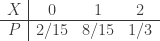
Thí dụ 2: Trong hộp có 10 sản phẩm trong đó có 6 chính phẩm. lấy ngẫu nhiên 2 sản phẩm, xây dựng quy luật phân phối xác suất của số chính phẩm được lấy ra.

Giải: Gọi X là: “số chính phẩm được lấy ra từ hộp” thì X là đại lượng ngẫu nhiên rời rạc có thể nhận các giá trị 0, 1, 2 với các xác suất tương ứng:

$P_1 = P(X = 0) = \dfrac{{C_4^2 }}{{C_{10}^2 }} = \dfrac{2}{{15}}$

$P_2 = P(X = 1) = \dfrac{{C_6^1 C_4^1 }}{{C_{10}^2 }} = \dfrac{8}{{15}}$

$P_3 = P(X = 2) = \dfrac{{C_6^2 }}{{C_{10}^2 }} = \dfrac{5}{{15}}$

Vậy quy luật phân phối xác suất của X là:

$\begin{array}{c| c c c } X & 0 & 1 & 2 \\ \hline P & 2/15 & 8/15 & 1/3 \\ \end{array}$

2. Hàm phân phối xác suất:

Hàm phân phối xác suất áp dụng cho cả đại lượng ngẫu nhiên rời rạc và liên tục.

Giả sử X là đại lượng ngẫu nhiên bất kỳ, x là một số thực nào đó. Xét biến cố “đại lượng ngẫu nhiên X nhận giá trị nhỏ hơn x”. Biến cố này được ký hiệu (X < x). Hiển nhiên là x thay đổi thì xác suất P(X < x) cũng thay đổi theo. Như vậy xác suất này là một hàm số của x.

a) Định nghĩa: Hàm phân phối xác suất của đại lượng ngẫu nhiên X, ký hiệu là F(x) là xác suất để đại lượng ngẫu nhiên nhận giá trị nhỏ hơn x, với x là một số thực bất kỳ.

$F(x) = P(X < x)$

Ta chú ý rằng đây là định nghĩa tổng quát của hàm phân phối xác suất. Đối với từng loại đại lượng ngẫu nhiên hàm phân phối xác suất được tính theo công thức riêng. Chẳng hạn nếu X là đại lượng ngẫu nhiên rời rạc thì hàm phân phối xác suất F(x) được xác định bằng công thức

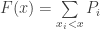$F(x) = \sum\limits_{x_i < x} {P_i }$ (1)

(Trong đó ký hiệu xi < x dưới dấu Σ có nghĩa là tổng này được lấy theo mọi trị số xi của đại lượng ngẫu nhiên bé hơn x).

Thí dụ: Tiến hành bắn 3 viên đạn độc lập. Xác suất trúng bia của mỗi viên bằng 0,4. Lập hàm phân phối của số lần trúng.

Giải: Gọi X là số lần trúng. X có thể nhận các giá trị: 0, 1, 2, 3. Với các xác suất tương ứng là:

$P_1 = P(X = 0) = (0,6)^3 = 0,216$

$P_2 = P(X =1) = C_{1}^{3}. 0,4.(0,6)^2 = 0,432$

$P_3 = P(X = 2) = C_2^3.(0,4)^2. 0,6 = 0,288$

$P_4 = P(X = 3) = (0,4)^3 = 0,064$

Ta có bảng phân phối xác suất của X:

$\begin{array}{c| c c c c } X & 0 & 1 & 2 & 3 \\ \hline P & 0,216 & 0,432 & 0,288 & 0,064 \\ \end{array}$

* Khi x = 0, biến cố (X < x) là biến cố không thể có do đó F(x) = 0

* Khi 0 < x = 1 biến cố (X < x) chỉ xảy ra khi X = 0 nên F(x) = P1 = 0,216

* Khi 0 < x = 2 biến cố (X < x) sẽ xảy ra khi X = 0 hoặc khi X = 1

Do đó: F(x) = P1 + P2 = 0,216 + 0,432 = 0,643

* Khi 2 < x = 3 ta có: F(x) = P1 + P2 + P3 = 0,216 + 0,432 + 0,288 = 0,936

* Khi x > 3 ta có: F(x) = P1 + P2 + P3 + P4 = 1

Vậy hàm phân phối xác suất có dạng:

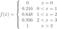
$f(x) = \left \{ \begin{array}{c c} 0 & x = 0 \\ 0.216 & 0 < x = 1 \\ 0.648 & 1 < x = 2 \\ 0.936 & 2 < x = 3 \\ 1 & x > 3 \\ \end{array} \right.$

Đồ thị của F(x) được biểu diễn trên hình (3.1).

Như vậy đồ thị hàm phân phối xác suất của đại lượng ngẫu nhiên rời rạc có dạng bậc thang với số điểm gián đoạn chính bằng số giá trị có thể có của X.

Nếu X là đại lượng ngẫu nhiên liên tục thì hàm phân phối xác suất của nó liên tục và khả vi tại mọi điểm của X, do đó đồ thị của nó là đường cong liên tục.

b/ Các tính chất của hàm phân phối xác suất:

Tính chất 1: Hàm phân phối xác suất F(x) luôn nhận giá trị giữa 0 và 1: 0 ≤ F(x) ≤1.

Tính chất này được trực tiếp suy từ định nghĩa của hàm phân phối xác suất, vì nó là một xác suất nên: 0 ≤ F(x) ≤1

Tính chất 2: Hàm phân phối xác suất là hàm không giảm; tức là nếu x₂ > x₁₂ ) ≥ F(x₁). thì F(x

Chứng minh: Giả sử x₂ > x₁ . Xét biến cố (X < x₂) biến cố này có thể phân tích thành hai biến cố xung khắc là ( X < x₁ ) và ( x₁ = X < x₂ ).

Theo định lý cộng xác suất ta có: P( X < x₂ ) = P( X < x₁ ) + P(x₁ = X < x₂ )

Hay F(x₂ ) – F(x₁ ) = P( x₁ = X < x₂ ) (3.2)

Song vế phải là một xác suất, nó luôn không âm do đó ta có: F(x₂ ) – F(x₁ ) ≥ 0

Vậy: F(x₂ ) ≥ F(x₁ ) ♦

Tính chất 3: Ta có biểu thức giới hạn sau: F(-∞) = 0; F(+∞) = 1.

Thật vậy: F(-∞) = P(X < -∞) = P(V) = 0; F(+∞) = P(X < +∞) = P(U) = 1

c) Các hệ quả:Từ các tính chất trên có thể suy ra một số hệ quả sau:

Hệ quả 1: Xác suất để đại lượng X nhận giá trị trong khoảng nửa kín bên trái [a, b) bằng hiệu các giá trị của hàm phân phối tại các nút: P(a = x < b) = F(b) – F(a).

Hệ quả này suy ra trực tiếp từ biểu thức (3.2) trong quá trình chứng minh tính chất 2.

Hệ quả 2: Xác suất để đại lượng ngẫu nhiên liên tục X nhận một giá trị xác định bằng 0: P(X=x) = 0.

Thật vậy, nếu đặt a = x, b = x + Δx, ta có: P(x = X < x + Δx) = F(x + Δx) – F(x).

Lấy giới hạn 2 vế khi Δx →0:

Vì X là đại lượng ngẫu nhiên liên tục do đó tại điểm x hàm phân phối xác suất cũng liên tục.

Vì vậy:

Do đó: P(X = x) = F(x) – F(x) = 0 ♦

Hệ quả 3: Đối với đại lượng ngẫu nhiên liên tục X ta có đẳng thức sau đây:

P(a ≤ X ≤ b) = P(a ≤ X < b) = P(a < X ≤ b) = P(a < X < b) = F(b) – F(a)

Chẳng hạn đẳng thức:

P(a ≤ X < b) = P(X = a) + P(a < X < b) = P(a < X < b)

Như vậy việc xét xác suất để đại lượng ngẫu nhiên liên tục X nhận một giá trị xác định là không có ý nghĩa, song việc tìm xác suất để nó nhận giá trị trong một khoảng lại rất có ý nghĩa.

d) Ý nghĩa của hàm phân phối xác suất:

Từ định nghĩa của hàm phân phối xác suất F(X) = P(X < x) ta thấy hàm phân phối xác suất phản ánh mức độ tập trung xác suất về phía bên trái của điểm x. Vì toàn bộ xác suất của đại lượng ngẫu nhiên bằng 1, do đó giá trị của hàm phân phối xác suất tại điểm x cho biết có bao nhiêu phần của một đơn vị xác suất phân phối trong khoảng (-∞, x)

3. Hàm mật độ xác suất:

a) Định nghĩa: Hàm mật độ xác suất của đại lượng ngẫu nhiên liên tục X ký hiệu là f(x) là đạo hàm bậc nhất của hàm phân phối xác suất của đại lượng ngẫu nhiên đó: f(x) = F’(x).

Từ định nghĩa trên ta thấy rằng hàm mật độ xác suất chỉ áp dụng được đối với đại lượng ngẫu nhiên liên tục vì chỉ trong trường hợp đó hàm phân phối xác suất F(x) mới liên tục và khả vi với mọi giá trị x.

b) Các tính chất của hàm mật độ xác suất:

Tính chất 1: Hàm mật độ xác suất luôn không âm: f(x) ≥ 0, với mọi x.

Chứng minh: Hàm phân phối xác suất F(x) là một hàm không giảm do đó đạo hàm của nó F’(x) = f(x) là một hàm không âm. Về mặt hình học điều đó có nghĩa là đồ thị của hàm f(x) không nằm thấp hơn trục Ox.

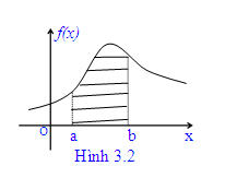
Tính chất 2: Xác suất để đại lượng ngẫu nhiên liên tục X nhận giá trị trong khoảng (a,b) bằng tích phân xác định của hàm mật độ xác suất trong khoảng đó:

Về mặt hình học, tính chất 2 được minh họa như sau:

Xác suất để đại lượng ngẫu nhiên liên tục X nhận giá trị trong khoảng (a, b) bằng diện tích của miền giới hạn bởi trục Ox, đường cong f(x) và các đường thẳng x = a, x = b (miền gạch trên hình 3.2).

Tính chất 3: Hàm phân phối xác suất F(x) của đại lượng ngẫu nhiên liên tục X bằng tích phân suy rộng của hàm mật độ xác suất trong khoảng (-∞; x).

Công thức trên cho phép tìm hàm phân phối xác suất của đại lượng ngẫu nhiên liên tục khi biết hàm mật độ xác suất của nó.

Về mặt hình học, công thức trên cho thấy giá trị của hàm phân phối xác suất F(x) tại điểm a bằng diện tích giới hạn bởi trục Ox, đường cong f(x) và đường thẳng x = a (miền gạch trên hình 3.3).

Tính chất 4: tích phân suy rộng trong khoảng (-∞;∞) của hàm mật độ xác suất bằng 1

Thí dụ: Hàm phân phối xác suất của đại lượng ngẫu nhiên liên tục X có dạng:

a) Tìm hệ số a. b) Tìm hàm mật độ xác suất f(x). c) Tìm xác suất để đại lượng ngẫu nhiên X nhận giá trị trong khoảng (0,2; 0,8).

Giải

a. Vì hàm phân phối xác suất F(x) là liên tục nên:

Do đó: a = 1

b. Theo định nghĩa hàm mật độ. Ta có:

c. Theo tính chất hàm phân phối xác suất:

P(0.2 < x < 0.8) = F(0.8) – F(0.2) = 0.504

III . MỘT SỐ QUY LUẬT PHÂN PHỐI XÁC SUẤT RỜI RẠC

1. Quy luật nhị thức B(n, p)

a) Bài toán:

Từ tập hợp gồm N phần tử trong đó có M phần tử có tính chất B nào đó, còn N-M phần tử không có tính chất B, ta lấy ngẫu nhiên có hoàn lại n phần tử. Nếu lấy theo phương thức này thì n phép thử nói trên sẽ độc lập với nhau vì việc lấy được phần tử có tính chất B, hay không có tính chất B trong mỗi lần lấy không ảnh hưởng đến khả năng lấy được phần tử có tính chất B hay không có tính chất B ở các lần lấy khác. Trong mỗi lần lấy chỉ có 2 trường hợp đối lập xảy ra. Hoặc biến cố A xảy ra (lấy được phấn tử có tính chất B) hoặc biến cố A không xảy ra (lấy được phần tử không có tính chất B).

Xác suất cho biến cố A xảy ra trong mỗi phép thử đều bằng $p = \dfrac{M}{N}$ xác suất cho biến cố A không xảy ra cũng đều bằng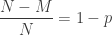 $\dfrac{N-M}{N} = 1 - p$

Gọi X là số lần biến cố A xảy ra trong n phép thử, thì X là đại lượng ngẫu nhiên rời rạc nhận các giá trị có thể có 0, 1, 2, …, n. Như đã chứng minh ở chương II, xác suất để X nhận các giá trị tương ứng được tính bằng công thức Bernoulli:

$P_x = P(X = x) = C_{n}^{x}{p^x}{(1-p)^{n-x}} (x = 0, 1, 2, ..., n)$ (1)

b) Định nghĩa: Đại lượng ngẫu nhiên rời rạc X nhận một trong các giá trị có thể có (x = 0, 1, …, n;) với các xác suất tương ứng được tính theo công thức (1) gọi là phân phối theo quy luật nhị thức với các tham số là n và p. Quy luật nhị thức được ký hiệu là B(n, p)

Nói cách khác, phân phối nhị thức gắn liền với việc lặp lại n lần một phép thử có hai sự kiện đối lập (thành công và thất bại; xảy ra và không xảy ra) với X là số lần thành công. Việc lặp lại ở đây có nghĩa là dãy phép thử được tiến hành trong cùng điều kiện và độc lập với nhau.

Như vậy bảng phân phối xác suất của đại lượng ngẫu nhiên X phân phối theo quy luật nhị thức có dạng:

$\begin{array}{c|cccccc} x & 0 & 1 & 2 & 3 & { \dots} & n \\ \hline P_x & {C_{n}^{0}{p^0}{q^n}} & {C_{n}^{1}{p^1}{q^{n-1}}} & {C_{n}^{2}{p^2}{q^{n-2}}} & {C_{n}^{3}{p^3}{q^{n-3}}} & { \dots} & {C_{n}^{n}{p^n}{q^{0}}} \\ \end{array}$

Trong thực tế, nhiều khi ta cần tính xác suất để đại lượng ngẫu nhiên X phân phối theo quy luật nhị thức (ký hiệu là X ~ B(n, p)) nhận giá trị trong khoảng [x, x + h] (với h nguyên dương và h ≤ n – x). Khi đó ta có thể tính xác suất này theo công thức:

$P(x \le X \le x + h) = P_x + P_{x+1} + ... + P_{x+h}$ (2)

Trong đó: $P_x, P_{x+1}, P_{x+h}$ được tính theo công thức (1).

Thật vậy biến cố (x ≤ X ≤ x + h) có thể tách thành tổng của h +1 biến cố xung khắc từng đôi là (X = x), (X = x +1), …, (X = x + h); do đó áp dụng định lý cộng xác suất với các biến cố đó ta có:

$P(x \le X \le x + h) \\ = P(X = x) + P(X = x +1) + ... + P(X = x + h) \\ = P_{x} + P_{x+1} + ... + P_{x+h}$ (3)

Ví dụ 1:Gieo 4 hạt đậu, xác suất để 1 hạt cho cây ra hoa vàng là 0.75, ra hoa trắng là 0.25. Số cây đậu ra hoa vàng X có phân phối nhị thức B(4;0.75)

Ta có:

$\begin{array}{c | c c c c c} x & 0 & 1 & 2 & 3 & 4 \\ \hline P & {0.25^4} & {4.0.75.0.25^3} & 6.{0.75}^2{0.25}^2 & {4.(0.75)^{3}.0.25} & {0.75^4} \\ \end{array}$

Ví dụ 2: Một phân xưởng có 5 máy hoạt động độc lập, xác suất để trong một ngày mỗi máy bị hỏng đều bằng 0,1. Tìm xác suất để:

a) Trong một ngày có 2 máy hỏng.

b) Trong một ngày có không quá 2 máy hỏng.

Giải:

Nếu coi sự hoạt động của mỗi máy là một phép thử, ta có 5 phép thử độc lập. Trong mỗi phép thử chỉ có 2 trường hợp: hoặc máy hỏng hoặc không. Xác suất hỏng của mỗi máy đều bằng 0,1. Gọi X là số máy hỏng trong một ngày thì X phân phối theo quy luật nhị thức với các tham số n = 5, p = 0,1 (tức là X ~ B(5; 0,1)).

Do đó xác suất để trong một ngày có 2 máy hỏng là xác suất để X = 2. Theo công thức (3.2) ta có:

$P(X = 2) = C_{5}^2(0,1)^2(0,9)^3 = 0,0729$

Xác suất để trong ngày có không quá 2 máy hỏng là xác suất để X nhận giá trị trong khoảng [0, 2]. Theo công thức (3.3) ta có:

$P(0 \le X \le 2) = P_{0} + P_{1} + P_{2}$

$P_0 = C_5^0.(0,1)^0(0,9)^5 = 0,59049$

$P_1 = C_5^1(0,1)^1(0,9)^4 = 0,32805$

Vậy: P(0 ≤ X ≤ 2) = 0,59049 + 0,32805 + 0,0729 = 0,99144

Ví dụ 3: Một học sinh làm bài trắc nghiệm có 100 câu, mỗi câu gồm có 4 phương án lựa chọn, trong đó có 1 phương án trả lời đúng. Với một câu, nếu học sinh đó trả lời đúng thì được 1 điểm, ngược lại, sẽ không có điểm. Do học sinh đó lười học nên không nắm được bài, đã làm bài bằng cách chọn đại 1 phương án trả lời. Tìm xác suất để học sinh đó đạt được kết quả (đạt 50 điểm trở lên)

Học sinh thực hiện bài trắc nghiệm trên chính là đã thực hiện 100 phép thử Bernoulli, với xác suất thành công là 0.25. Gọi X là số điểm của học sinh đó thì X ~ B(100;0.25)

Tuy nhiên, ở đây ta không thể làm như ví dụ 2, vì xác suất của biến cố học sinh đạt kết quả tương đương với xác suất P( X ≥ 50). Vì việc liệt kê và tính từng trường hợp X = 50, 51, 52, …, 100 tốn rất nhiều thời gian.

Trong thực tế khi số phép thử n khá lớn, việc sử dụng các công thức (2) và (3) gặp nhiều khó khăn. Trong trường hợp này, người ta thường sử dụng các công thức gần đúng để tính toán.

Khi n khá lớn, xác suất p không quá gần 0 và không quá gần 1, ta có thể áp dụng công thức tích phân Laplace xấp xỉ như sau:

$P_x = C_n^x.p^xq^{n-x} \approx { \dfrac{1}{\sqrt{npq}}} f({ \dfrac{x-np}{\sqrt{npq}}})$ (4)

trong đó 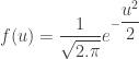$f(u) = { \dfrac{1}{\sqrt{2.{\pi}}}} e^{-{ \dfrac{u^2}{2}}}$ gọi là hàm Gauss

Nhận xét:

1. Để tính giá trị của các hàm f(u), chúng ta có thể tra các giá trị hàm Laplace được tính sẵn ở các bảng phụ lục (thông thường các sách XSTK đều có bảng phụ lục này).

2. Dễ dàng nhận thấy hàm f(u) là hàm chẵn, do đó f(-u) = f(u), nên thông thường các bảng phụ lục chỉ ghi các giá trị ứng với u ≥ 0.

3. Hầu hết các bảng phụ lục chỉ tính f(u) với u ≤ 5. Với u > 5 thì hàm f(u) giảm rất chậm và nhận giá trị gần bằng 0. Do vậy ta có thể lấy f(u) = 0 (với mọi u > 5).

3. Từ công thức trên ta cũng có công thức xấp xỉ:

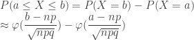
$P(a \le X \le b) = P(X=b) - P(X = a) \\ \approx {\varphi}({ \dfrac{b - np}{\sqrt{npq}}}) - {\varphi}({ \dfrac{a - np}{\sqrt{npq}}})$

trong đó 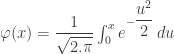${\varphi}(x) = { \dfrac{1}{\sqrt{2.{\pi}}}} \int_0^x e^{-{ \dfrac{u^2}{2}}} \, du$ (hàm Laplace). Hàm Laplace là hàm lẻ, với x > 5, hàm Laplace tăng rất chậm và nhận giá trị xấp xỉ bằng 0.5.

Quay lại ví dụ 3 ở trên, ta sẽ áp dụng công thức tích phân Lapplace để tính xác suất học sinh đó đạt yêu cầu. Rõ ràng:

$P(X \ge 50) = P(50 \le X \le 100) \\ \approx {\varphi} ( { \dfrac{100 - 100.(0.25)}{\sqrt{100.(0.25).(0.75)}}}) - {\varphi} ( { \dfrac{50 - 100.(0.25)}{\sqrt{18.75}}})$

Hay: $P(X \ge 50) \approx {\varphi}(17.32) - {\varphi}(5.77) \approx 0.5 - 0.5 \approx 0$

Khi xác suất p ≈ 0 (rất bé) ta sử dụng định lý sau:

Định lý Poisson:

Cho X ~ B(n;p).

Khi $n \to + \infty , p \to 0 , np = \lambda (const)$

Thì $\lim_{n \to +{\infty}} P_n(k) = { \dfrac{e^{- {\lambda}}{\lambda}^k}{k!}}$

Nghĩa là: khi n khá lớn và p khá nhỏ, n.p = const thì:

$P_{n}(k) \approx { \dfrac{e^{-{ \lambda}}.{ \lambda}^k}{k!}}$

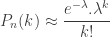
Ví dụ: Xác suất gặp một thứ phẩm trong một lô hàng áo sơ mi cao cấp là 0,003. Tìm xác suất để gặp 8 thứ phẩm trong 1000 sản phẩm đó.

Giải: Do n = 1000 , p = 0,003 ≈ 0 → λ = np = 3

Gọi X là số thứ phẩm trong 1000 sản phẩm thì X ~ B(1000;0,003). Tuy nhiên do n lớn và p khá nhỏ nên ta áp dụng công thức tính xấp xỉ Poisson.

Ta có: $P[X=8] \approx { \dfrac{e^{-3}.3^8}{8!}} \approx 0,0081$

Các ví dụ tương tự:

1. Một cuốn sách có 500 trang, mỗi trang có hơn 300 chữ. Biết cuốn sách đó có 300 chữ in sai. Mở ngẫu nhiên 1 trang. Tìm xác suất để trang đó có 3 chữ in sai. Đ/s: 0.0198

2. Trong 1 đợt xổ số, người ta phát hành 100.000 vé, trong đó có 10.000 vé trúng giải. Nếu 1 người mua 10 vé thì xác suất trúng ít nhất 1 vé là bao nhiêu? Đ/s: 0,76

3.Một trạm cho thuê xe du lịch có 3 chiếc xe. Hàng ngày, trạm phải nộp tiền trả góp 500.000đ cho 1 chiếc xe (bất kể xe đó có được thuê hay không). Mỗi chiếc được cho thuê với giá 1.500.000 đ /ngày.

Giả sử số xe được yêu cầu cho thuê của trạm trong 1 ngày là đại lượng ngẫu nhiên X có phân phối nhị thức B(3;0.8).

a.Tính số tiền trung bình trạm thu được trong 1 ngày.

b. Giải bài toán trên trong trường hợp trạm có 4 chiếc xe. Theo bạn, trạm nên có 3 hay 4 chiếc xe?

4. Xác suất để gặp 1 laptop bị lỗi là 0,005. Tìm xác suất để khi chọn ngẫu nhiên 1000 laptop ta gặp:

a. 10 máy bị lỗi. Đ/s: 0.018

b. Có không quá 5 máy bị lỗi Đ/s:0.61596

5. Trong một đợt thi nâng bậc thợ của ngành dệt, mỗi công nhân dự thi sẽ chọn ngẫu nhiên 1 trong 2 máy và với máy đã chọn dệt 100 sản phẩm.

Nếu trong 100 sản phẩm sản xuất ra có từ 75 sản phẩm loại 1 trở lên thì được nâng bậc.

Giả sử đối với công nhân A, xác suất để sản xuất được sản phẩm loại 1 đối với 2 máy lần lượt là 0.7 và 0.8.

Tính xác suất để công nhân được nâng bậc thợ. Đ/s: 0.5161

Gửi bình luận

Tháng Sáu 29, 2009

Mean value theorem

Filed under: Bài viết lượm lặt, Giải tích — tranthevu @ 11:23 sáng

http://en.wikipedia.org/wiki/Mean_value_theorem
Formal statement
Let f : [a, b] → R be a continuous function on the closed interval [a, b], and differentiable on the open interval (a, b), where a < b. Then there exists some c in (a, b) such that

$f^{'}(c) = \frac{f(b)-f(a)}{b-a}$ .

The mean value theorem is a generalization of Rolle's theorem, which assumes f(a) = f(b), so that the right-hand side above is zero.

The mean value theorem is still valid in a slightly more general setting. One only needs to assume that f : [a, b] → R is continuous on [a, b], and that for every x in (a, b) the limit

$\lim_{h\to 0}\frac{f(x+h)-f(x)}{h}$

exists as a finite number or equals +∞ or −∞. If finite, that limit equals f' (x). An example where this version of the theorem applies is given by the real-valued cube root function mapping x to x1/3, whose derivative tends to infinity at the origin.

Note that the theorem is false if a differentiable function is complex-valued instead of real-valued. Indeed, define $f(x) = e^{ix}$ for all real x. Then

$f(2π)−f(0) =0=0(2π−0)$ ,

while

$|f'(x)|=1$ .
Proof
The expression (ƒ(b) − ƒ(a)) / (b − a) gives the slope of the line joining the points (a, ƒ(a)) and (b, ƒ(b)), which is a chord of the graph of ƒ, while ƒ ′(x) gives the slope of the tangent to the curve at the point (x, ƒ(x)). Thus the Mean value theorem says that given any chord of a smooth curve, we can find a point lying between the end-points of the chord such that the tangent at that point is parallel to the chord. The following proof illustrates this idea.

Define g(x) = ƒ(x) − rx, where r is a constant. Since ƒ is continuous on [a, b] and differentiable on (a, b), the same is true of g. We now want to choose r so that g satisfies the conditions of Rolle’s theorem. Namely

$\begin{align}g(a)=g(b)&\Leftrightarrow f(a)-ra=f(b)-rb\\&\Leftrightarrow r=\frac{f(b)-f(a)}{b-a}\cdot\end{align}$

By Rolle’s theorem, since g is continuous and g(a) = g(b), there is some c in (a, b) for which g ′(c) = 0, and it follows from the equality g(x) = ƒ(x) − rx that,

$f '(c)=g '(c)+r=0+r=\frac{f(b)-f(a)}{b-a}$

as required.
A simple application
Assume that f is a continuous, real-valued function, defined on an arbitrary interval I of the real line. If the derivative of f at every interior point of the interval I exists and is zero, then f is constant.

Proof: Assume the derivative of f at every interior point of the interval I exists and is zero. Let (a, b) be an arbitrary open interval in I. By the mean value theorem, there exists a point c in (a,b) such that

$0 = f'(c) = \frac{f(b)-f(a)}{b-a}$

This implies that f(a) = f(b). Thus, f is constant on the interior of I and thus is constant on I by continuity. (See below for a multivariable version of this result.)

Remarks:

* Only continuity of ƒ, not differentiability, is needed at the endpoints of the interval I. No hypothesis of continuity needs to be stated if I is an open interval, since the existence of a derivative at a point implies the continuity at this point. (See the section continuity and differentiability of the article derivative.)
* The differentiability of ƒ can be relaxed to one-sided differentiability, a proof given in the article on semi-differentiability.
Cauchy’s mean value theorem
Cauchy’s mean value theorem, also known as the extended mean value theorem, is the more general form of the mean value theorem. It states: If functions f and g are both continuous on the closed interval [a,b], and differentiable on the open interval (a, b), then there exists some c ∈ (a,b), such that
$(f(b)-f(a))g\,'(c)=(g(b)-g(a))f\,'(c).\$ ,

Of course, if g(a) ≠ g(b) and if g′(c) ≠ 0, this is equivalent to:

$\frac{f'(c)}{g'(c)}=\frac{f(b)-f(a)}{g(b)-g(a)}\cdot$

Geometrically, this means that there is some tangent to the graph of the curve

$\begin{array}{ccc}[a,b]&\longrightarrow&\mathbb{R}^2\\t&\mapsto&\bigl(f(t),g(t)\bigr),\end{array}$

which is parallel to the line defined by the points (f(a),g(a)) and (f(b),g(b)). However Cauchy’s theorem does not claim the existence of such a tangent in all cases where (f(a),g(a)) and (f(b),g(b)) are distinct points, since it might be satisfied only for some value c with f′(c) = g′(c) = 0, in other words a value for which the mentioned curve is stationary; in such points no tangent to the curve is likely to be defined at all. An example of this situation is the curve given by

$t\mapsto(t^3,1-t^2)$ ,

which on the interval [−1,1] goes from the point (−1,0) to (1,0), yet never has a horizontal tangent; however it has a stationary point (in fact a cusp) at t = 0.

Proof of Cauchy’s mean value theorem
Cauchy’s mean value theorem can be used to prove l’Hôpital’s rule. The mean value theorem is the special case of Cauchy’s mean value theorem when g(t) = t.

The proof of Cauchy’s mean value theorem is based on the same idea as the proof of the mean value theorem. First we need to define a new function that satisfies the conditions of Rolle’s theorem. Define the function h by

$h(x)=\bigl(f(b)-f(a)\bigr)\bigl(g(x)-g(a)\bigr)-\bigl(g(b)-g(a)\bigr)\bigl(f(x)-f(a)\bigr)$ ,

which is continuous on [a,b] and differentiable on (a, b). Then

$h(a)=\bigl(f(b)-f(a)\bigr)\bigl(g(a)-g(a)\bigr)-\bigl(g(b)-g(a)\bigr)\bigl(f(a)-f(a)\bigr)=0$

and

$h(b)=\bigl(f(b)-f(a)\bigr)\bigl(g(b)-g(a)\bigr)-\bigl(g(b)-g(a)\bigr)\bigl(f(b)-f(a)\bigr)=0$ ,

so h(a) = h(b) and Rolle’s theorem applies. The derivative of h is

$h^{'}(x)=\bigl(f(b)-f(a)\bigr)g^{'}(x) - \bigl(g(b)-g(a)\bigr)f^{'}(x)$

and Rolle’s theorem states that it is equal to zero at some point, i.e., h'(c)=0 for some c ∈ (a, b). The equation for the derivative at c is

$h^{'}(c)=\bigl(f(b)-f(a)\bigr)g^{'}(c) - \bigl(g(b)-g(a)\bigr)f^{'}(c)=0$ ,

therefore

$\bigl(f(b)-f(a)\bigr)g^{'}(c) = \bigl(g(b)-g(a)\bigr)f^{'}(c)$ .

If $g^{'}(c)$ and $g(b)−g(a)$ are nonzero this can be written as

$\frac{f^{'}(c)}{g^{'}(c)} = \frac{f(b)-f(a)}{g(b)-g(a)}$ .
Mean value theorem in several variables
The mean value theorem in one variable generalizes to several variables by applying the theorem in one variable via parametrization. Let G be an open subset of Rn, and let ƒ : G → R be a differentiable function. Fix points x, y ∈ G such that the interval x y lies in G, and define $g(t) = f((1 − t)x + ty)$ . Since g is a differentiable function in one variable, the mean value theorem gives:

$g(1)−g(0) = g^{'}(c)$

for some c between 0 and 1. But since g(1) = f(y) and g(0) = f(x), computing g'(c) explicitly we have:

$f(y) - f(x) = \nabla f ((1- c)x + cy) \cdot (y - x)$

where \nabla denotes a gradient and \cdot a dot product. Note that this is an exact analog of the theorem in one variable (in the case n=1 this is the theorem in one variable). By the Schwarz inequality, the equation gives the estimate:

$|f(y) - f(x)| \le |\nabla f ((1- c)x + cy)| \, |y - x|$ .

In particular, when the partial derivatives of ƒ are bounded, ƒ is Lipschitz continuous (a fortiori, uniformly continuous). Note that ƒ is not assumed to be continuously differentiable nor continuous on the closure of G. However, in the above, we used the chain rule so the existence of \nabla f would not be sufficient.

As an application of the above, we prove that ƒ is constant if G is connected and every partial derivative of ƒ is 0. Pick some point x_0 \in G, and let g(x) = f(x) − f(x0). We want to show g(x) = 0 for every x \in G. For that, let E = \{ x \in G | g(x) = 0 \}. Then E is closed and nonempty. It is open too: for every x ∈ E,

$|g(y)| = |g(y) - g(x)| \le (0) |y - x| = 0$

for every y in some neighborhood of x. (Here, it is crucial that x and y are sufficiently close to each other.) Since G is connected, we conclude E = G.

Remark that all arguments in the above are made in a coordinate-free manner; hence, they actually generalize to the case when G is a subset of a Banach space.
Mean value theorem for vector-valued functions
There is no exact analog of the mean value theorem for vector-valued functions. The problem is roughly speaking the following: If f:U\rightarrow\mathbb{R}^m is a differentiable function (where U\subset\mathbb{R}^n is open) and if x+th,\,x,h\in\mathbb{R}^n,\,t\in[0,1] is the line segment in question (lying inside \,U), then one can apply the above parametrization procedure to each of the component functions f_i \, (i=1,\ldots,m) of \,f (in the above notation set \,y=x+h). In doing so one finds points \,x+t_ih on the line segment satisfying

$f_i(x+h) - f_i(x) = \nabla f_i (x + t_ih) \cdot h.\$ ,

But generally there will not be a single point \,x+t^* h on the line segment satisfying

$f_i(x+h) - f_i(x) = \nabla f_i (x + t^* h) \cdot h.\$ ,

for all \,i simultaneously. (As a counterexample one could take f:[0,2\pi]\rightarrow\mathbb{R}^2 defined via the component functions \,f_1(x)=\cos x, \,f_2(x)=\sin x. Then f(2\pi)-f(0)=0 \,(\in\mathbb{R}^2), but \,f_1′(x)=-\sin x and \,f_2′(x)=\cos x are never simultaneously zero as \, x ranges over \,[0,2\pi].)

However a certain type of generalization of the mean value theorem to vector-valued functions is obtained as follows: Let f be a continuously differentiable real-valued function defined on an open interval I, and let x as well as x + h be points of I. The mean value theorem in one variable tells us that there exists some \,t^* between 0 and 1 such that

$f(x+h)-f(x) = f'(x+t^*h)\cdot h. \$ ,

On the other hand we have

$f(x+h)-f(x) = \int_x^{x+h} f'(u)du = \left(\int_0^1 f'(x+th)\,dt\right)\cdot h$ .

Thus, the value f\,'(x+t^*h) at the particular point \,t^* has been replaced by the mean value \int_0^1 f'(x+th)\,dt. This last version can be generalized to vector valued functions:

Let U\subset\mathbb{R}^n be open, f:U\rightarrow\mathbb{R}^m continuously differentiable, and x\in U,\,h\in\mathbb{R}^n vectors such that the whole line segment x+th,\, 0\leq t\leq 1 remains in \,U. Then we have:

$\text{(*)} \qquad f(x+h)-f(x) = \left(\int_0^1 Df(x+th)\,dt\right)\cdot h$ ,

where the integral of a matrix is to be understood componentwise. (Dƒ denotes the Jacobian matrix of ƒ.)

From this one can further deduce that if ||Dƒ(x + th)|| is bounded for t between 0 and 1 by some constant M, then

$\text{(**)} \qquad ||f(x+h)-f(x)|| \leq M||h||$ .

Proof of (*). Write f_i\, (i=1,\ldots,m) for the real valued components of \,f. Define the functions g_i:[0,1]\rightarrow\mathbb{R} by g_i(t)\, :=\, f_i(x+th).

Then we have

$f_i(x+h)-f_i(x)\, =\, g_i(1)-g_i(0) =\int_0^1 g_i'(t)dt = \int_0^1 \left(\sum_{j=1}^n \frac{\partial f_i}{\partial x_j} (x+th)h_j\right)\,dt =\sum_{j=1}^n \left(\int_0^1 \frac{\partial f_i}{\partial x_j}(x+th)\,dt\right)h_j$ .

The claim follows since \,Df is the matrix consisting of the components \frac{\partial f_i}{\partial x_j}, q.e.d.

Proof of (**). From (*) it follows that $||f(x+h)-f(x)||=||\int_0^1 (Df(x+th)\cdot h)\,dt|| \leq \int_0^1 ||Df(x+th)|| \cdot ||h||\, dt \leq M||h||$ .

Here we have used the following

Lemma. Let v:[a,b]\rightarrow\mathbb{R}^m be a continuous function defined on the interval $[a,b]\subset\mathbb{R}$ . Then we have

$'\text{(***)}\qquad ||\int_a^b v(t)\,dt||\leq \int_a^b ||v(t)||\,dt$ .

Proof of (***). Let $u\in\mathbb{R}^m$ denote the value of the integral $u:=\int_a^b v(t)\,dt$ . Now

$||u||^2 = \langle u,u \rangle = \left\langle \int_a^b v(t) dt,u \right\rangle = \int_a^b \langle v(t),u \rangle \,dt \leq \int_a^b ||v(t)||\cdot ||u||\,dt = ||u|| \int_a^b ||v(t)||\,dt$ ,

thus ||u|| \leq \int_a^b ||v(t)||\,dt as desired. (Note the use of the Cauchy-Schwarz inequality.) This shows (***) and thereby finishes the proof of (**).
Mean value theorems for integration
First mean value theorem for integration

The first mean value theorem for integration states

If G : [a, b] → R is a continuous function and φ : [a, b] → [0, ∞) is an integrable function, then there exists a number x in [a, b] such that

$\int_a^b G(t)\varphi (t) \, dt=G(x) \int_a^b \varphi (t) \, dt$ .

In particular, if φ(t) = 1 for all t in [a, b], then there exists x in [a, b] such that

$\int_a^b G(t) \, dt=\ G(x)(b - a).\$ ,

[edit] Proof of the first mean value theorem for integration

It follows from the extreme value theorem that the continuous function G has a finite infimum m and a finite supremum M on the interval [a, b]. From the monotonicity of the integral and the fact that m ≤ G(t) ≤ M, it follows that

$m I\le \int^b_aG(t)\varphi(t) \, dt \le M I$ ,

where

$I:=\int^b_a\varphi(t) \, dt$

denotes the integral of φ. Hence, if I = 0, then the claimed equality holds for every x in [a, b]. Therefore, we may assume I > 0 in the following. Dividing through by I we have that

$m \le \frac1I\int^b_aG(t)\varphi(t) \, dt\le M$ .

The extreme value theorem tell us more than just that the infimum and supremum of G on [a, b] are finite; it tells us that both are actually attained. Thus we can apply the intermediate value theorem, and conclude that the continuous function G attains every value of the interval [m, M], in particular there exists x in [a, b] such that

$G(x) = \frac1I\int^b_aG(t)\varphi(t) \, dt$ .

This completes the proof.

Second mean value theorem for integration

There are various slightly different theorems called the second mean value theorem for integration. A commonly found version is as follows:

If G : [a, b] → R is a positive monotonically decreasing function and φ : [a, b] → R is an integrable function, then there exists a number x in (a, b] such that

$\int_a^b G(t)\varphi(t)\,dt = G(a+0) \int_a^x \varphi(t)\,dt$

\ Here G(a + 0) stands for ${\underset{a_+}{\lim}G}$ , the existence of which follows from the conditions. Note that it is essential that the interval (a, b] contains b. A variant not having this requirement is:

If G : [a, b] → R is a monotonic (not necessarily decreasing and positive) function and φ : [a, b] → R is an integrable function, then there exists a number x in (a, b) such that

$\int_a^b G(t)\varphi(t)\,dt = G(a+0) \int_a^x \varphi(t)\,dt + G(b-0) \int_x^b \varphi(t)\,dt$ .

This variant was proved by Hiroshi Okamura in 1947

Gửi bình luận

Tháng Sáu 12, 2009

Wiener process

Filed under: Bài viết lượm lặt — Thẻ:wiener — tranthevu @ 10:22 sáng

Characterizations of the Wiener process

The Wiener process $W_t$ is characterized by three facts:

1. $W_0 = 0$
2. $W_t$ is almost surely continuous
3. $W_t$ has independent increments with distribution $W_t-W_s\sim \mathcal{N}(0,t-s)$ (for 0 ≤ s ≤ t).

$N(\mu, \sigma ^{2})$ denotes the normal distribution with expected value $\mu$ and variance $\sigma ^{2}$ . The condition that it has independent increments means that if 0 ≤ s1 ≤ t1 ≤ s 2 ≤ t2 then $W_{t_{1}}-W_{s_{1}}$ and $W_{t_{2}}-W_{s_{2}}$ are independent random variables, and the similar condition holds for $n$ increments.

An alternative characterization of the Wiener process is the so-called Lévy characterization that says that the Wiener process is an almost surely continuous martingale with $W_0 = 0$ and quadratic variation $[W_t, W_t] = t$ (which means that $W_{t}^{2}-t$ is also a martingale).

A third characterization is that the Wiener process has a spectral representation as a sine series whose coefficients are independent $N(0,1)$ random variables. This representation can be obtained using the Karhunen-Loève theorem.

The Wiener process can be constructed as the scaling limit of a random walk, or other discrete-time stochastic processes with stationary independent increments. This is known as Donsker's theorem. Like the random walk, the Wiener process is recurrent in one or two dimensions (meaning that it returns almost surely to any fixed neighborhood of the origin infinitely often) whereas it is not recurrent in dimensions three and higher. Unlike the random walk, it is scale invariant, meaning that

$\alpha^{-1}W_{\alpha^2 t}\$ ,

is a Wiener process for any nonzero constant $\alpha$ . The Wiener measure is the probability law on the space of continuous functions $g$ , with $g(0) = 0$ , induced by the Wiener process. An integral based on Wiener measure may be called a Wiener integral.

Properties of a one-dimensional Wiener process

Basic properties

The unconditional probability density function at a fixed time $t$ :

$f_{W_t}(x) = \frac{1}{\sqrt{2 \pi t}} e^{-x^2/{2 t} }$ .

The expectation is zero:

$E(W_t) = 0$ .

The variance is $t$ :

$E(W^2_t) - E^2(W_t) = t$ .

The covariance and correlation:

${cov}(W_s,W_t) = \min(s,t) \,$ ,

${corr}(W_s,W_t) = \frac{\min(s,t)}{\sqrt{st}} = \sqrt{ \frac{ \min(s,t) }{ \max(s,t) } } \,$ .

The results for the expectation and variance follow immediately from the definition that increments have a normal distribution, centred at zero. Thus

$W_t = W_t-W_0 \sim \mathcal{N}(0,t)$ .

The results for the covariance and correlation follow from the definition that non-overlapping increments are independent, of which only the property that they are uncorrelated is used. Suppose that $t_1 0$ the process $V_t = (1/\sqrt c) W_{ct}$ is another Wiener process.

Time reversal

The process $V_{t}=W_{1}-W_{1-t}$ for 0 ≤ t ≤ 1 is distributed like $W_t$ for 0 ≤ t ≤ 1.

Time inversion

The process $V_t = tW_1 / t$ is another Wiener process.

A class of Brownian martingales

If a polynomial $p(x,t)$ satisfies the PDE

$\Big( \frac{\partial}{\partial t} + \frac12 \frac{\partial^2}{\partial x^2} \Big) p(x,t) = 0$

then the stochastic process

$M_t = p ( W_t, t ) \,$

is a martingale.

Example: $W_{t}^{2}-t$ is a martingale, which shows that the quadratic variation of $W$ on $[0,t]$ is equal to $t$ . It follows that the expected time of first exit of $W$ from $(-c,c)$ is equal to $c^2$ .

More generally, for every polynomial p(x,t) the following stochastic process is a martingale:

$M_t = p ( W_t, t ) - \int_0^t a(W_s,s) \, \mathrm{d}s \,$ ,

where a is the polynomial

$a(x,t) = \Big( \frac{\partial}{\partial t} + \frac12 \frac{\partial^2}{\partial x^2} \Big) p(x,t) \,$ .

Example: $p(x,t)=(x^{2}-t)^{2}$ , $a(x,t) = 4{x^2}$ ; the process $(W_t^2 - t)^2 - 4 \int_0^t W_s^2 \,$ $\mathrm{d}s$ is a martingale, which shows that the quadratic variation of the martingale $W_t^2 - t$ on $[0,t]$ is equal to $4 \int_0^t W_s^2 \, \mathrm{d}s$ .

About functions $p(x,t)$ more general than polynomials, see local martingales.

Some properties of sample paths

The set of all functions w with these properties is of full Wiener measure. That is, a path (sample function) of the Wiener process has all these properties almost surely.

Qualitative properties

* For every ε>0, the function w takes both (strictly) positive and (strictly) negative values on (0,ε).

* The function $w$ is continuous everywhere but differentiable nowhere (like the Weierstrass function).

* Points of local maximum of the function $w$ are a dense countable set; the maximum values are pairwise different; each local maximum is sharp in the following sense: if $w$ has a local maximum at $t$ then $|w(s)-w(t)|/|s-t| \to \infty$ as $s$ tends to $t$ . The same holds for local minima.

* The function $w$ has no points of local increase, that is, no t>0 satisfies the following for some ε in $(0,t)$ : first, $W(s)\leq W(t)$ for all s in (t-ε,t), and second, $W(s)\geq W(t)$ for all s in (t,t+ε). (Local increase is a weaker condition than that $w$ is increasing on (t-ε,t+ε).) The same holds for local decrease.

* The function $w$ is of unbounded variation on every interval.

* Zeros of the function $w$ are a nowhere dense perfect set of Lebesgue measure 0 and Hausdorff dimension 1/2.

Quantitative properties

Law of the iterated logarithm

$\limsup_{t\to+\infty} \frac{ |w(t)| }{ \sqrt{ 2t \log\log t } } = 1$ .

Modulus of continuity

Local modulus of continuity:

$\limsup_{\varepsilon\to0+} \frac{ |w(\varepsilon)| }{ \sqrt{ 2\varepsilon \log\log(1/\varepsilon) } } = 1$ .

Global modulus of continuity (Lévy):
$\limsup_{\varepsilon\to0+} \sup_{0\le s<t\le 1, t-s\le\varepsilon} \frac{ |w(s)-w(t)| }{ \sqrt{ 2\varepsilon \log(1/\varepsilon) } } = 1$ .

Local time

The image of the Lebesgue measure on $[0,t]$ under the map $w$ (the pushforward measure) has a density $L_{t}(.)$ . Thus,

$\int_0^t f(w(s)) \, \mathrm{d}s = \int_{-\infty}^{+\infty} f(x) L_t(x) \, \mathrm{d}x$
for a wide class of functions $f$ (namely: all continuous functions; all locally integrable functions; all non-negative measurable functions). The density Lt is (more exactly, can and will be chosen to be) continuous. The number $L_{t}(x)$ is called the local time at $x$ of $w$ on $[0,t]$ . It is strictly positive for all $x$ of the interval $(a,b)$ where a and b are the least and the greatest value of $w$ on $[0,t]$ , respectively. (For $x$ outside this interval the local time evidently vanishes.) Treated as a function of two variables $x$ and $t$ , the local time is still continuous. Treated as a function of $t$ (while $x$ is fixed), the local time is a singular function corresponding to a nonatomic measure on the set of zeros of $w$ .

These continuity properties are fairly non-trivial. Consider that the local time can also be defined (as the density of the pushforward measure) for a smooth function. Then, however, the density is discontinuous, unless the given function is monotone. In other words, there is a conflict between good behavior of a function and good behavior of its local time. In this sense, the continuity of the local time of the Wiener process is another manifestation of non-smoothness of the trajectory.

Related processes
The generator of a Brownian motion is ½ times the Laplace-Beltrami operator. The image above is of the Brownian motion on a special manifold: the surface of a sphere.

The stochastic process defined by

$X_t = \mu t + \sigma W_t \,$

is called a Wiener process with drift $\mu$ and infinitesimal variance $\sigma ^{2}$ . These processes exhaust continuous Lévy processes.

Two random processes on the time interval $[0,1]$ appear, roughly speaking, when conditioning the Wiener process to vanish on both ends of $[0,1]$ . With no further conditioning, the process takes both positive and negative values on $[0,1]$ and is called Brownian bridge. Conditioned also to stay positive on $(0,1)$ , the process is called Brownian excursion. In both cases a rigorous treatment involves a limiting procedure, since the formula $P(A|B) = P(A\cap B) / P(B)$ does not work when $P(B) = 0$ .

A geometric Brownian motion can be written

$e^{[\beta t-(\alpha^2 t/2)+\alpha W_t]}.\,$

It is a stochastic process which is used to model processes that can never take on negative values, such as the value of stocks.

The stochastic process

${ X_t = \mathrm{e}^{-t} W_{\mathrm{e}^{2t}} }$

is distributed like the Ornstein–Uhlenbeck process

The time of hitting a single point $x > 0$ by the Wiener process is a random variable with the Lévy distribution. The family of these random variables (indexed by all positive numbers $x$ ) is a left-continuous modification of a Lévy process. The right-continuous modification of this process is given by times of first exit from closed intervals $[0,x]$ .

The local time $L_{t}(0)$ treated as a random function of t is a random process distributed like the process $S_t = \max_{0\le s\le t} W_s$ .

The local time $L_{t}(x)$ treated as a random function of $x$ (while $t$ is constant) is a random process described by Ray-Knight theorems in terms of Bessel processes.

Brownian martingales

Let A be an event related to the Wiener process (more formally: a set, measurable with respect to the Wiener measure, in the space of functions), and Xt the conditional probability of A given the Wiener process on the time interval [0, t] (more formally: the Wiener measure of the set of trajectories whose concatenation with the given partial trajectory on [0, t] belongs to A). Then the process Xt is a continuous martingale. Its martingale property follows immediately from the definitions, but its continuity is a very special fact – a special case of a general theorem stating that all Brownian martingales are continuous. A Brownian martingale is, by definition, a martingale adapted to the Brownian filtration; and the Brownian filtration is, by definition, the filtration generated by the Wiener process.

Time change

Every continuous martingale (starting at the origin) is a time changed Wiener process.

Example. $2W_t=V(4t)$ where V is another Wiener process (different from $W$ but distributed like $W$ ).

Example. $W_t^2 - t = V_{A(t)}$ where $A(t) = 4 \int_0^t W_s^2 \, \mathrm{d} s$ and $V$ is another Wiener process.

In general, if $M$ is a continuous martingale then $M_{t}-M_{0}=V_{A(t)}$ where $A(t)$ is the quadratic variation of $M$ on $[0,t]$ , and $V$ is a Wiener process.

Corollary. (See also Doob's martingale convergence theorems) Let Mt be a continuous martingale, and

$M^-_\infty = \liminf_{t\to\infty} M_t, \quad M^+_\infty = \limsup_{t\to\infty} M_t$ .

Then only the following two cases are possible:

$-\infty < M^-_\infty = M^+_\infty < +\infty, \quad -\infty = M^-_\infty < M^+_\infty = +\infty$ ;

other cases (such as $M^-_\infty = M^+_\infty = +\infty, M^-_\infty < M^+_\infty < +\infty etc$ .) are of probability $0$ .

Especially, a nonnegative continuous martingale has a finite limit (as $t\to\infty$ ) almost surely.

All stated (in this subsection) for martingales holds also for local martingales.

+Change of measure

A wide class of continuous semimartingales (especially, of diffusion processes) is related to the Wiener process via a combination of time change and change of measure.

Using this fact, the qualitative properties stated above for the Wiener process can be generalized to a wide class of continuous semimartingales.

Complex-valued Wiener process

The complex-valued Wiener process may be defined as a complex-valued random process of the form $Z_t = X_t + iY_t$ where Xt,Yt are independent Wiener processes (real-valued).

Self-similarity

Brownian scaling, time reversal, time inversion: the same as in the real-valued case.

Rotation invariance: for every complex number $c$ such that $|c|=1$ the process $cZ_t$ is another complex-valued Wiener process.

+Time change

If $f$ is an entire function then the process $f(Z_{t})-f(0)$ is a time-changed complex-valued Wiener process.

Example. $Z_t^2 = (X_t^2-Y_t^2) + 2 X_t Y_t \mathrm{i} = U_{A(t)}$ where $A(t) = 4 \int_0^t |Z_s|^2 \, \mathrm{d}s$ and $U$ is another complex-valued Wiener process.

In contrast to the real-valued case, a complex-valued martingale is generally not a time-changed complex-valued Wiener process. For example, the martingale $2X_t + iY_t$ is not (here $X_t$ , $Y_t$ are independent Wiener processes, as before).
link :
http://en.wikipedia.org/wiki/Wiener_measure

Gửi bình luận

Tháng Sáu 11, 2009

Phương sai

Filed under: Bài viết lượm lặt, Xác suất — Thẻ:phương sai, variance — tranthevu @ 10:53 chiều

Định nghĩa

Nếu $\mu = {E}(X)$ là giá trị kỳ vọng của biến ngẫu nhiên X, thì phương sai là

${var}(X) = E( {( X - \mu ) ^ 2} )$ .

Nghĩa là, phương sai là giá trị kỳ vọng của bình phương của độ lệch của X so với giá trị trung bình của nó. Nói nôm na, phương sai là “trung bình của bình phương khoảng cách của mỗi điểm dữ liệu tới trung bình”. Do đó, nó là giá trị trung bình của bình phương độ lệch. Phương sai của biến ngẫu nhiên X thường được ký hiệu là $var(X), \sigma_X^2$ , hoặc đơn giản là $\sigma^2$ .

Lưu ý: định nghĩa trên áp dụng cho cả các biến ngẫu nhiên rời rạc và liên tục.

Nhiều phân phối, ví dụ như phân phối Cauchy, là không có phương sai, do tích phân có được từ định nghĩa phương sai là phân kỳ. Một phân phối không tồn tại giá trị kỳ vọng thì cũng không tồn tại phương sai. Nhưng điều ngược lại thì không đúng: có những phân phối mà giá trị kì vọng tồn tại nhưng không tồn tại phương sai.
Các tính chất

* Nếu phương sai tồn tại, thì nó không bao giờ âm, vì bình phương một số luôn dương hoặc bằng 0.
* Đơn vị của phương sai là bình phương đơn vị của giá trị quan sát được của biến ngẫu nhiên. Ví dụ, phương sai của tập hợp các chiều cao đo được tính theo centimet (cm) có đơn vị là cm bình phương. Đơn vị này gây bất tiện nên các nhà thống kê thường sử dụng căn bậc hai của phương sai, gọi là độ lệch chuẩn, coi như là tổng của các phân tán.
* Nếu a và b là các hằng số thực, X là một biến ngẫu nhiên, thì aX + b cũng là biến ngẫu nhiên với phương sai là:

$var(aX+b)=a^2{var}(X)$ .

* Khi tính phương sai, để thuận tiện ta thường dùng công thức:

$var(X)= E(X^2 - 2XE(X) + (E(X))^2) = E(X^2) - 2{(E(X))}^2 + {(E(X))}^2 = E(X^2) - {(E(X))}^2$ .

* ${var}(aX+bY) =a^2 {var}(X) + b^2 {var}(Y) + 2ab {cov}(X, Y)$ .

Với ${cov}$ là hiệp phương sai, bằng 0 nếu X và Y là 2 biến ngẫu nhiên độc lập lẫn nhau.

Xấp xỉ phương sai của một hàm số

Phương pháp Delta sử dụng khai triển Taylor bậc hai để xấp xỉ phương sai của hàm số của một hay nhiều biến ngẫu nhiên. Ví dụ, phương sai của hàm số theo một biến ngẫu nhiên được xấp xỉ bởi:

${var}\left[f(X)\right]\approx \left(f'({E}\left[X\right])\right)^2{var}\left[X\right]$

với giả thiết $f(\cdot)$ khả vi bậc hai, trung bình và phương sai của X là hữu hạn (tức tồn tại).

Phương sai của tổng thể chung và phương sai mẫu

Trên nhiều tình huống thực tế, giá trị chính xác của phương sai của một tổng thể, kí hiệu bởi σ2 là không thể xác định trước được.

Phương pháp chung để ước lượng phương sai của một tổng thể (hữu hạn hoặc vô hạn) là ta sẽ lấy một mẫu hữu hạn các cá thể từ quần thể. Giả sử rằng mẫu thu được có các giá trị đo được là $x_1,\dots,x_N$ .

Phương sai của mẫu (gọi tắt là phương sai mẫu) $(x_1,\dots,x_N)$ , được tính bởi:

$\hat{\sigma}^2 = \frac{1}{N} \sum_{i=1}^N \left(x_i - \overline{x} \right)^ 2$ ,

trong đó $\overline{x}$ là số bình quân số học của mẫu.

Tuy nhiên, $\hat{\sigma^2}$ là một ước lượng chệch (biased) của phương sai quần thể. Ước lượng sau là một ước lượng không chệch (unbiased) của phương sai quần thể:

$s^2 = \frac{1}{N-1} \sum_{i=1}^N \left(x_i - \overline{x} \right)^ 2$ ,

Chứng minh 1

Phần sau đây chứng minh $s^2$ là một ước lượng không chệch của phương sai quần thể. Một ước lượng $\hat{\theta}$ của tham số $\theta$ được gọi là ước lượng không chệch nếu ${E}\{ \hat{\theta}\} = \theta$ .

Kí hiệu μ và $\theta^2$ lần lượt là trung bình và phương sai của quần thể. Để chứng minh $s^2$ là ước lượng không chệch, ta sẽ chứng minh rằng $E{ s^2} = \sigma^2$ . Ta có:

$E (s^2) = E \left\{ \frac{1}{n-1} \sum_{i=1}^n \left( x_i - \overline{x} \right) ^ 2 \right\}$

$= \frac{1}{n-1} \sum_{i=1}^n E \left\{ \left( x_i - \overline{x} \right) ^ 2 \right\}$

$= \frac{1}{n-1} \sum_{i=1}^n {E} \left\{ \left( (x_i - \mu) - (\overline{x} - \mu) \right) ^ 2 \right\}$

$= \frac{1}{n-1} \sum_{i=1}^n \left\{ {E} \left\{ (x_i - \mu)^2 \right\} - 2 E \left\{ (x_i - \mu) (\overline{x} - \mu) \right\} + {E} \left\{ (\overline{x} - \mu) ^ 2 \right\} \right\}$

$= \frac{1}{n-1} \sum_{i=1}^n \left\{ \sigma^2 - 2 \left( \frac{1}{n} \sum_{j=1}^n {E} \left\{ (x_i - \mu) (x_j - \mu) \right\} \right) + \frac{1}{n^2} \sum_{j=1}^n \sum_{k=1}^n {E} \left\{ (x_j - \mu) (x_k - \mu) \right\} \right\}$

$= \frac{1}{n-1} \sum_{i=1}^n \left\{ \sigma^2 - \frac{2 \sigma^2}{n} + \frac{\sigma^2}{n} \right\}$

$= \frac{1}{n-1} \sum_{i=1}^n \frac{(n-1)\sigma^2}{n}$

$= \frac{(n-1)\sigma^2}{n-1} = \sigma^2$

Chứng minh 2

Ta cũng có thể chứng minh bằng cách sau:

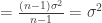
$E\left[ \sum_{i=1}^n {(x_i-\overline{x})^2}\right] =E\left[ \sum_{i=1}^n {x_i^2}\right] - nE[ \overline{x}^2]$

$=nE[x_i^2] - \frac{1}{n} E\left[\left(\sum_{i=1}^n x_i\right)^2\right]$

$=n({var}[x_i] + (E[x_i])^2) - \frac{1}{n} E\left[\left(\sum_{i=1}^n x_i\right)^2\right]$

$=n\sigma^2 + \frac{1}{n}(nE[x_i])^2 - \frac{1}{n}E\left[\left(\sum_{i=1}^n x_i\right)^2\right]$

$=n\sigma^2 - \frac{1}{n}\left( E\left[\left(\sum_{i=1}^n x_i\right)^2\right] - \left(E\left[\sum_{i=1}^n x_i\right]\right)^2\right)$

$=n\sigma^2 - \frac{1}{n}\left({var}\left[\sum_{i=1}^n x_i\right]\right) =n\sigma^2 - \frac{1}{n}(n\sigma^2) =(n-1)\sigma^2$ .

Phương sai của véc tơ ngẫu nhiên

Nếu $X$ là một véc tơ ngẫu nhiên, xác định trên $R^n$ , thì phương sai của $X$ được xác định bởi:

$E[(X-\mu )(X-\mu )^{T}]$

với $\mu$ = $E(X)$ và $X^T$ là ma trận chuyển vị của $X$ . Phương sai này là một ma trận vuông xác định dương. Nó thường được gọi là ma trận hiệp phương sai.

Comments (1)

Dirac Measure

Filed under: Bài viết lượm lặt — Thẻ:dirac, dirac measure, độ đo dirac — tranthevu @ 11:03 sáng

Let $X$ be a nonempty set. Let $P(X)$ denote the power set of $X$ .Then $(X,P(X))$ is a measurable space.

Let $x\in X$ The Dirac measure concentrated at $x$ is $\delta _{x}:P(X)\rightarrow \{0,1\}$ defined by

$\delta _{x}(E)= 1$ if $x\in E$ , $\delta _{x}(E)= 0$ if $x\not\in E$

Note that the Dirac measure $\delta _{x}$ is indeed a measure

1.Since $x\not\in E$ we have $\delta _{x}(\emptyset )=0$

2.If Ann is a sequence of pairwise disjoint subsets of X then one of the following must happen:

+ $x\not\in \cup _{n\in N}A_{n}$ in which case $\delta _{x}(\cup _{n\in N}A_{n})=0$ and $\delta _{x}(A_{n})=0$ for every $n\in N$

+ $x\in \cup _{n\in N}A_{n}$ in which case $x\in A_{n_{0}}$ for exactly one $n_{0}\in N$ causing $\delta _{x}(\cup _{n\in N}A_{n})=1$ , $\delta _{x}(A_{n_{0}})=1$ and $\delta _{x}(A_{n})=1$ for every $n \in N$ and $n\not=n_{0}$ .

Also $(X,P(X),\delta _{x})$ note that is a probability space.

Let $\overline{R}$ denote the extended real numbers. Then for any function $f$ : $X\rightarrow \overline{R}$ the integral of $f$ with respect to the Dirac measure $\delta _{x}$ is

$\int\limits_{X}fd\delta _{x}=f(x)$

If $X=R$ denotes Lebesgue measure, $A$ is a Lebesgue measurable subset of $R$ and $\delta$ (no subscript) denotes the Dirac delta function, then for any measurable function $f: R\rightarrow R$ we have

$\int\limits_{A}\delta (t-x)f(t)m(t)=\int\limits_{A}fd\delta_{x}=f(x)\delta _{x}(A)$

Moreover, if $f$ is defined so that $f(t)=1$ for all $t\in A$ the above equation becomes

$\int\limits_{A}\delta (t-x)m(t)=\int\limits_{A}d\delta _{x}=\delta _{x}(A)$

In other words, integration with respect to the Dirac measure $\delta_{x}$ amounts to evaluating the function at $x$

In other words, the function (with $x \in R$ ) fixed and t a real variable) behaves like a Radon-Nikodym derivative of $\delta _{x}$ with respect to m

Note that, just as the Dirac delta function is a misnomer (it is not really a function), there is not really a Radon-Nikodym derivative of $\delta _{x}$ with respect to $m$ since $\delta _{x}$ is not absolutely continuous with respect to $m$

Gửi bình luận

Cauchy Distribution

Filed under: Bài viết lượm lặt — Thẻ:cauchy, cauchy distribution, phân bố caushy — tranthevu @ 6:00 sáng

The Cauchy distribution, also called the Lorentzian distribution or Lorentz distribution, is a continuous distribution describing resonance behavior. It also describes the distribution of horizontal distances at which a line segment tilted at a random angle cuts the x-axis.

Let represent the angle that a line, with fixed point of rotation, makes with the vertical axis, as shown above. Then

			(1)
			(2)
			(3)
			(4)

so the distribution of angle is given by

(5)

This is normalized over all angles, since

(6)

and

			(7)
			(8)
			(9)

The general Cauchy distribution and its cumulative distribution can be written as

			(10)
			(11)

where is the half width at half maximum and is the statistical median. In the illustration about, .

The Cauchy distribution is implemented in Mathematica as CauchyDistribution[m, Gamma/2].

The characteristic function is

			(12)
			(13)

The moments of the distribution are undefined since the integrals

(14)

diverge for .

If and are variates with a normal distribution, then has a Cauchy distribution with statistical median and full width

(15)

The sum of variates each from a Cauchy distribution has itself a Cauchy distribution, as can be seen from

		$F_t^(-1){[phi(t)]^n}(x)$	(16)
			(17)

where is the characteristic function and is the inverse Fourier transform, taken with parameters

Gửi bình luận

Tháng Sáu 10, 2009

Linear Least Square Problem and Singular Value Decomposition (SVD)

Filed under: Bài viết lượm lặt — Thẻ:SVD — tranthevu @ 4:41 chiều

Linear Least Square Problem (linear least squares), or ordinary least squares (OLS), is an important computational problem, that arises primarily in applications when it is desired to fit a linear mathematical model to measurements obtained from experiments. The goals of linear least squares are to extract predictions from the measurements and to reduce the effect of measurement errors. Mathematically, it can be stated as the problem of finding an approximate solution to an overdetermined system of linear equations. In statistics, it corresponds to the maximum likelihood estimate for a linear regression with normally distributed error.

Linear least square problems admit a closed-form solution, in contrast to non-linear least squares problems, which often have to be solved by an iterative procedure.

Motivational example

As a result of an experiment, four (x,y) data points were obtained, (1,6) , (2,5) , (3,7) , and (4,10) (shown in red in the picture on the right). It is desired to find a line $y = \beta_1 + \beta_2x$ that fits “best” these four points. In other words, we would like to find the numbers $\beta_1$ and $\beta_2$ that approximately solve the overdetermined linear system

$\begin{gathered} {\beta _1} + 1{\beta _2} = 6, \hfill \\ {\beta _1} + 2{\beta _2} = 5, \hfill \\ {\beta _1} + 3{\beta _...$

of four equations in two unknowns in some “best” sense.

The least squares approach to solving this problem is to try to make as small as possible the sum of squares of “errors” between the right- and left-hand sides of these equations, that is, to find the minimum of the function

$S(\beta_1, \beta_2)= \left[6-(\beta_1+1\beta_2)\right]^2 +\left[5-(\beta_1+2\beta_2) \right]^2 +\left[7-(\beta_1 + 3\beta_2)\...$

The minimum is determined by calculating the partial derivatives of $S(\beta_1,\beta_2)$ in respect to $\beta_1$ and $\beta_2$ and setting them to zero. This results in a system of two equations in two unknowns, called the normal equations, which, when solved, gives the solution

$\beta_1 = 3.5$ , $\beta_2 = 1.4$

and the equation y = 3.5 + 1.4x of the line of best fit. The residuals, that is, the discrepancies between the values from the experiment and the values calculated using the line of best fit are then found to be 1.1 , -1.3 , -0.7 , and 0.9 (see the picture on the right). The minimum value of the sum of squares is

S(3.5,1.4) = 1.12 + (-1.3)2 + (-0.7)2 + 0.92 = 4.2 .

The general problem

Consider an overdetermined system (there are more equations than unknowns)

$\sum_{j=1}^{n} X_{ij}\beta_j = y_i,\ (i=1, 2, \dots, m),$

of linear equations in unknown coefficients, $\beta_1,\beta_2,...,\beta_n$ , with m > n , written in matrix form as $\mathbf {X} \boldsymbol {\beta} = \mathbf {y},$ where

$\mathbf {X}=\begin{pmatrix} X_{11} & X_{12} & \cdots & X_{1n} \\ X_{21} & X_{22} & \cdots & X_{2n} \\...$

Such a system usually has no solution, and the goal is then to find the coefficients $\beta$ which fit the equations “best”, in the sense of solving the quadratic minimization problem

$\mathop {\rm argmin}\limits_\beta \sum\limits_{i = 1}^m {{{\left| {{y_i} - \sum\limits_{j = 1}^n {{X_{ij}}} {\beta _j}} \rig...$

A justification for choosing this criterion is given in properties below. This minimization problem has a unique solution, provided that the n columns of the matrix are linearly independent, given by solving the normal equations

$(\mathbf X^\top \mathbf X )\hat \boldsymbol \beta= \mathbf X^\top \mathbf y.$

Singular value decomposition

In linear algebra, the singular value decomposition (SVD) is an important factorization of a rectangular real or complex matrix, with many applications in signal processing and statistics. Applications which employ the SVD include computing the pseudoinverse, least squares fitting of data, matrix approximation, and determining the rank, range and null space of a matrix.

Suppose is an -by- matrix whose entries come from the field , which is either the field of real numbers or the field of complex numbers. Then there exists a factorization of the form

$M = U\Sigma V^*,$

where is an -by- unitary matrix over , the matrix $\Sigma$ is -by- diagonal matrix with nonnegative real numbers on the diagonal, and V^* denotes the conjugate transpose of , an -by- unitary matrix over . Such a factorization is called a singular-value decomposition of . A common convention is to order the diagonal entries $\Sigma_{i,i}$ in non-increasing fashion. In this case, the diagonal matrix $\Sigma$ is uniquely determined by (though the matrices and are not). The diagonal entries of $\Sigma$ are known as the singular values of .

In practice, matrix consists of eigenvectors of matrix AA^T while matrix consists of eigenvectors of matrix A^TA . Finally, matrix $\Sigma$ is the square root of a diagonal matrix forming by eigenvalues of either matrix AA^T or matrix A^TA .

Example

Let us consider the case when

$A = \left( {\begin{array}{*{20}{c}} 2 & 4 \\ 1 & 3 \\ 0 & 0 \\ 0 & 0 \\ \end{array} ...$

Having yields

$A{A^T} = \left( {\begin{array}{*{20}{c}} {20} & {14} & 0 & 0 \\ {14} & {10} & 0 & 0 \\ 0 &...$

By simple calculation, one has

$\lambda_1=15+\sqrt{221}, \quad \lambda_2 =15-\sqrt{221}$

being eigenvalues of matrix A^TA (in the descending form), which helps us to write down

$\Sigma = \left( {\begin{array}{*{20}{c}} {15 + \sqrt {221} } & 0 \\ 0 & {15 - \sqrt {221} } \\ 0 & 0 ...$

To construct matrix , one has to find eigenvectors corresponding to eignvalues $\lambda_1$ and $\lambda_2$ . For the first one, that is, $\lambda_1$ , one has the following linear system

$\left( {\begin{array}{*{20}{c}} { - 10 - \sqrt {221} } & {11} \\ {11} & {10 - \sqrt {221} } \\ \end{array} ...$

which implies, for example,

${x_1} = \frac{{11}} {{\sqrt {442 + 20\sqrt {221} } }}, \quad {x_2} = \frac{{10 + 221}} {{\sqrt {442 + 20\sqrt {221} } }}.$

Similar to $\lambda_2$ , one has its corresponding eigenvector as follows

${x_3} = \frac{{11}} {{\sqrt {442 - 20\sqrt {221} } }}, \quad {x_4} = \frac{{10 - 221}} {{\sqrt {442 - 20\sqrt {221} } }}.$

Thus

$V = \left( {\begin{array}{*{20}{c}} {\frac{{11}} {{\sqrt {442 + 20\sqrt {221} } }}} & {\frac{{11}} {{\sqrt {442 - 20\s...$

The numerical solution of is

$V = \left( {\begin{array}{*{20}{c}} {{\text{0}}{\text{.4045535848}}} & {{\text{0}}{\text{.9145142955}}} \\ {{\text...$

which gives us

${V^T}V = \left( {\begin{array}{*{20}{c}} {{\text{1}}{\text{.000000000}}} & {{\text{ - }}{\text{.4e - 9}}} \\ {{\te...$

Having we can compute by the following formula $U=AV\Sigma^{-1}$ or you can perform the same routine as above. That is

$U = \left( {\begin{array}{*{20}{c}} {{\text{0}}{\text{.1495732296}}} & {{\text{1}}{\text{.574048236}}} & 0 & 0...$ .

It is easy to see that

$U\Sigma {V^T} = \left( {\begin{array}{*{20}{c}} {{\text{1}}{\text{.999999783}}} & {{\text{4}}{\text{.000000099}}} \\ ...$

Having a SVD result, that is

$A = U\left( {\begin{array}{*{20}{c}} {{\Sigma _1}} \\ 0 \\ \end{array} } \right){V^T}$

one can see that the solution of Ax=b can be computed by $x = V\left( {\begin{array}{*{20}{c}} {\Sigma _1^{ - 1}} & 0 \\ \end{array} } \right){U^T}b.$ Note that matrices and are not unique. Using Maple software, you can compute SVD as shown below.